Self-Learning

1. Semi-supervised Learning

기존 기계학습은 각각의 데이터 x에 대한 Target Label y가 제공되는지에 대한 여부로 Supervised Learning과 Unsupervised Learning으로 나눌 수 있습니다. Supervised Learning에 있어서 Label은 현재 구축하려는 모델 혹은 알고리즘이 지향할 목표이자 정답 역할을 하기에 필수 불가결합니다.
하지만 Label이 있는 데이터를 구하는 것은 언제나 쉬운 일이 아닙니다. Label이 있는 데이터를 다루는 데 있어서 가장 큰 문제는 믿을 수 있는 라벨을 얻기 위해선 시간과 노력이 지나치게 많이 들어갈 수 있다는 점에 있습니다.
다시 원점으로 돌아오면, 왜 굳이 unlabeled data를 기계학습에 참여하게 해야 하는 걸까요? 시간과 노력이 엄청나게 들어감에도 불구하고?

• 이유는 다음과 같습니다.

a) labeled data에 비해서 unlabeled data는 그 수가 비교도 안 되게 많으며, 쉽게 구할 수 있다.

b) 기존 labeled data로 훈련된 모델보다 훨씬 일반적인 모델 설계가 가능해진다.

(다만 언제나 도움이 되지는 않을 수도 있죠.)

Semi-supervised Learning이란?

: Labeled data와 unlabeled data를 모두 사용하여, 하나의 일반화된 모델을 만들어 내는 기계학습 방법.

• 하지만 여기서 혼동하지 말아야 할 하나의 개념을 더 소개하기로 하겠습니다.

Tranductive Learning?

: Semi-supervised와 동의어로 쓰이기도 하지만, 전반적인 모델을 만들기보다는 unlabeled data에 label을 붙이는 것에 초점을 맞추는 방법을 칭합니다.

• 각 기계학습 기법의 세부적인 비교는 아래 표를 참조하시기 바랍니다.

2. Self-Training 이론

self-training이란 앞서 소개한 semi-supervised learning의 한 갈래입니다.

self-training은 대략적으로 다음과 같은 방식으로 진행됩니다.

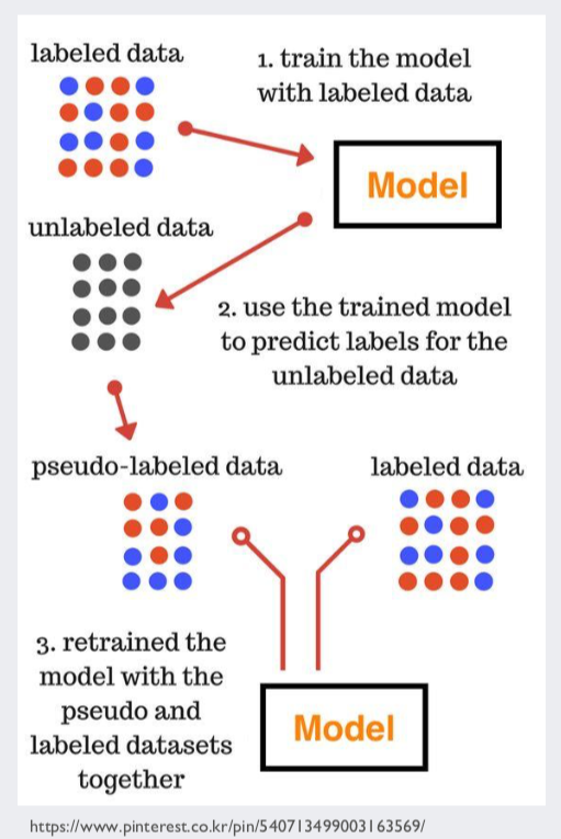
labeled data로 훈련한 모델로 unlabeled data의 label을 예측하고, 예측된 label을 정답으로 가정하여 훈련 데이터에 추가한 뒤, 다시 모델을 훈련시켜 나가는 것입니다.

• 그러나 무조건 현재 모델의 예측이 옳다고 가정하는 것은 문제가 있습니다.

따라서, 다음과 같은 변이를 주기도 합니다.

a) 모든 unlabeled data와 예측한 label을 훈련 데이터에 추가

b) 예측 결과값이 높게 나온 일부 unlabeled data의 라벨만 추가

c) 예측 결과값에 따라 가중치를 부여하여 추가

• 각 방식의 차이는 차후 코드를 통해 자세히 확인해보고자 합니다.
  
  훈련 모델을 활용하는 방법 이외에 clustering을 기반으로 하는 방법도 있습니다.

Propagating 1 Nearest Neighbor 방식은 비슷한 label을 갖는 데이터는 서로 거리가 가까이 위치한다는 가정에서 시작합니다.

• 해당 알고리즘은 대략적으로 다음과 같은 방식으로 진행됩니다.

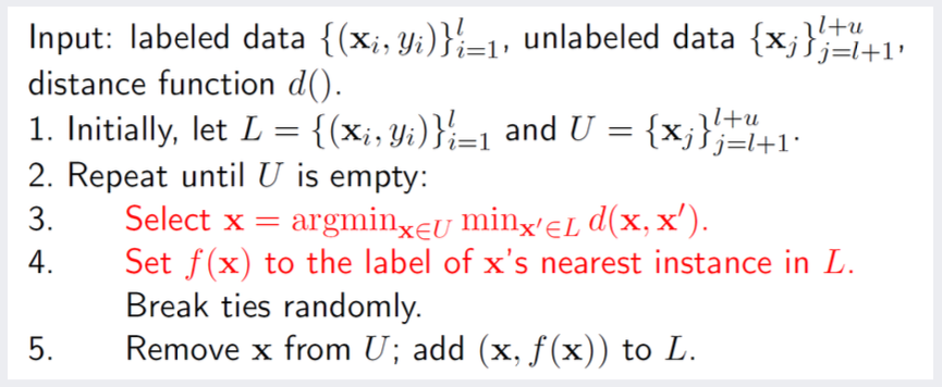
: unlabeled data 하나를 다른 labeled data 사이의 거리를 비교하여, 가장 가까운 거리에 위치한 data의 label을 부여하는 방법입니다.

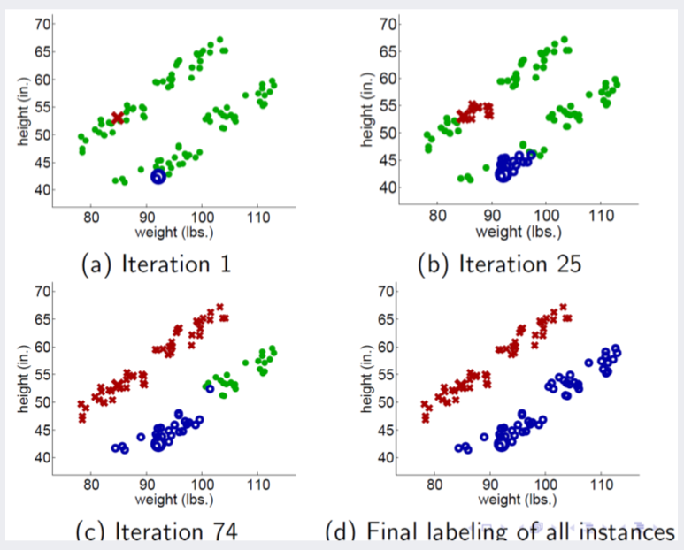
• 다음과 같이 데이터가 분류되는 것을 볼 수 있습니다.

하지만 해당 알고리즘은 outlier에 취약하다는 단점을 갖고 있습니다.

• 아래 그림은 outlier에 의해 오분류되는 사례를 가리킵니다.

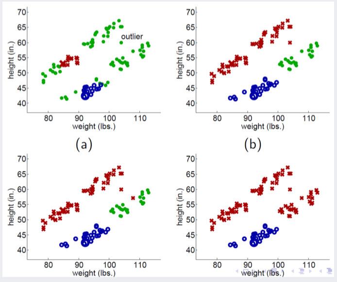
• 마찬가지로 자세한 알고리즘의 전개 과정은 코드 부분에서 살펴보겠습니다.

3. Self-Training 코드

• self-training 코드는 Tensorflow Tutorial에서 제공하는 MNIST 데이터와 기본 코드를 기반으로 작성하였습니다.

import tensorflow as tf
import numpy as np

# load mnist dataset
mnist = tf.keras.datasets.mnist
(x_train, y_train),(x_test, y_test) = mnist.load_data()
x_train, x_test = x_train / 255.0, x_test / 255.0

# convert label to one-hot vector
y_train = np.eye(10)[y_train]
y_test = np.eye(10)[y_test]

# shuffle train data
np.random.seed(0)
shuffled_indices = np.random.permutation(np.arange(6000))
x_train_shuffled = x_train[shuffled_indices, :, :]
y_train_shuffled = y_train[shuffled_indices, :]

# split train data into labeled / unlabeled data
x_labeled = x_train_shuffled[:50000, :, :]
y_labeled = y_train_shuffled[:50000, :]

x_unlabeled = x_train_shuffled[50000:, :, :]
y_unlabeled = y_train_shuffled[50000:, :]

# build simple nerual network
# 2 layers (256, 10 for nodes each, relu and softmax for activation, adam optimizer)
model = tf.keras.models.Sequential([
  tf.keras.layers.Flatten(),
  tf.keras.layers.Dense(256, activation=tf.nn.relu),
  tf.keras.layers.Dense(10, activation=tf.nn.softmax)
])
model.compile(optimizer='adam',
              loss='categorical_crossentropy',
              metrics=['accuracy'])

# train model (about 3 epochs)
model.fit(x_labeled, y_labeled, epochs=3)

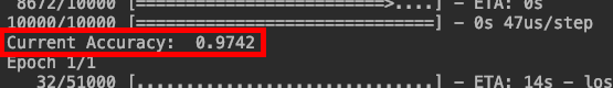
# obtain current accuracy
loss, acc = model.evaluate(x_test, y_test)
print("Current Accuracy: ", acc)

다음은 50000개의 sample로만 훈련한 결과입니다. self-training을 통해 test error가 어떻게 변화하는지 살펴보고자 합니다.

• 모델 기반 방식에는 세 가지 변이가 있었습니다.

a) 모든 unlabeled data와 예측한 label을 훈련 데이터에 추가

# add prediction of current model inferred from unlabeled data
if method == "all":

    # epochs
    for _ in range(2):
        # obtain prediction
        predictions = model.predict(x_unlabeled)

        # switch prediction to one-hot label
        pseudo_labels = np.argmax(predictions, axis=1)
        pseudo_labels = np.eye(10)[pseudo_labels]

        # concatenate all data
        all_x = np.concatenate([x_labeled, x_unlabeled], axis=0)
        all_y = np.concatenate([y_labeled, pseudo_labels], axis=0)

        # do fitting
        model.fit(all_x, all_y, epochs=1)

    # calculate test loss
    t_loss, t_acc = model.evaluate(x_test, y_test)

    print("Accuracy changed to : ", t_acc)

b) 예측 결과값이 높게 나온 일부 unlabeled data의 라벨만 추가

elif method == "top":

    # epochs
    for _ in range(2):

        # obtain prediction
        predictions = model.predict(x_unlabeled)

        # get prediction probability and its predicted label
        prediction_prob = np.amax(predictions, axis=1, keepdims=True)
        prediction_labels = np.argmax(predictions, axis=1)

        # sort logit into order
        prediction_sort = np.argsort(prediction_prob, axis=0)

        # get 1000 high probability instances
        index_target = np.where(prediction_sort < 1000)[0]

        # convert 1000 instances prediction to one-hot labels
        pseudo_labels_topten = prediction_labels[index_target]
        pseudo_labels_topten = np.eye(10)[pseudo_labels_topten]

        # top 1000 instances of x data
        x_unlabeled_topten = x_unlabeled[index_target, :, :]

        # concatenate data
        new_x = np.concatenate((x_labeled, x_unlabeled_topten), axis=0)
        new_y = np.concatenate((y_labeled, pseudo_labels_topten), axis=0)

        # do fitting
        model.fit(new_x, new_y, epochs=1)

    # calculate test loss
    t_loss, t_acc = model.evaluate(x_test, y_test)

    print("Accuracy changed to : ", t_acc)

c) 예측 결과값에 따라 가중치를 부여하여 추가

# apply weights for each predicted instances
elif method == "weight":

    # epochs
    for _ in range(2):

        # obtain predictions
        predictions = model.predict(x_unlabeled)

        # treat predicted logit as weight value
        pseudo_weights = np.amax(predictions, axis=1, keepdims=True)

        # convert weight as y vectors
        pseudo_labels = np.where(predictions == pseudo_weights, pseudo_weights, 0)

        # concatenate all data
        all_x = np.concatenate((x_labeled, x_unlabeled), axis=0)
        all_y = np.concatenate((y_labeled, pseudo_labels), axis=0)

        # do fitting
        model.fit(all_x, all_y, epochs=1)

    # calculate loss
    t_loss, t_acc = model.evaluate(x_test, y_test)

    print("Accuracy changed to : ", t_acc)

크지 않지만 확실하게 test accuracy가 증가하는 모습을 확인할 수 있었습니다.

• 이번에는 I-NN 기법을 확인해보겠습니다.

  두 개의 분포를 각각 하나의 instance를 기반으로 label을 부여하는 과정을 코드로 작성했습니다.

import math
import numpy as np
import matplotlib.pyplot as plt

# formulate two distribution with random noise
np.random.seed(0)
sample_num = np.arange(20)
x1 = 2*sample_num + 3*np.random.randn(20)
x2 = 3*sample_num + 40 + 2*np.random.randn(20)

# extract one instance from each distribution with label
labeled_data = [[[15, x1[15]],0], [[5, x2[5]],1]]

# make array of other data as unlabeled
unlabeled_data = [[i, x1[i]] for i in sample_num if i != 15]
unlabeled_data.extend([[i, x2[i]] for i in sample_num if i != 5])

unlabeled_data = np.array(unlabeled_data)

# shuffle unlabeled
np.random.shuffle(unlabeled_data)

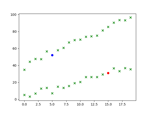
# plot current data distribution
plt.scatter(unlabeled_data[:, 0], unlabeled_data[: , 1], marker='x', color='g')
plt.plot(15, x1[15], marker='o', color='r')
plt.plot(5, x2[5], marker='o', color='b')
plt.show()

• 아래는 for-loop를 반복하며 라벨을 부여하는 과정을 코드로 작성한 것입니다.

# for each single unlabeled data
for single_u in unlabeled_data:

    # calculate distance to nearby labeled data
    distances_a = []
    distances_b = []

    # for all labeeld data
    for single_l in labeled_data:

        # calcualte L2 distance
        dist = math.sqrt((single_u[0]-single_l[0][0])**2 + (single_u[1]-single_l[0][1])**2)

        # calcualte distances with labels
        if single_l[1] == 0:
            distances_a.append(dist)
        else:
            distances_b.append(dist)

    # compare distances and give label of minimum fistnace
    if min(distances_a) < min(distances_b):
        labeled_data.append([single_u, 0])

    elif min(distances_a) > min(distances_b):
        labeled_data.append([single_u, 1])

    # break tie
    else:
        labeled_data.append([single_u, int(round(np.random.rand(1)[0]))])

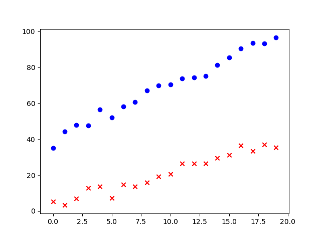
# plot the result
pseudo_x1 = np.array([i[0] for i in labeled_data if i[1] == 0])
pseudo_x2 = np.array([i[0] for i in labeled_data if i[1] == 1])

plt.scatter(pseudo_x1[:, 0], pseudo_x1[:,1], marker="x", color="r")
plt.scatter(pseudo_x2[:, 0], pseudo_x2[:,1], marker="o", color="b")
plt.show()

• 위에 작성한 코드는 다음 github repo(https://github.com/KYJun/self_training)에서 확인할 수 있습니다.

4. 정리

• 현재까지 Semi-supervised Learning과 그 한 갈래인 self-training 방식을 살펴보았습니다.

• Self-training의 장점과 단점은 다음과 같습니다.

• 장점

1) 무척 단순하다.

2) Wrapper 방식으로, 기존 분류 모델을 그대로 활용할 수 있다.

3) NLP (Natural Language Processing)와 같은 실제 사례에서도 활용된다.

• 단점

1) Outlier와 같은 데이터 상의 문제에 취약하다.

2) Convergence가 원활히 해결되지 못한다.

Reference

• 강필성 교수님 비즈니스 애널리틱스 05 semi-supervised Learning pdf
• https://www.tensorflow.org/tutorials/keras/basic_classification

Twitter  facebook  Google+